Rachael's Blog

Week 15 – Predicting Loan Defaults

Well, the end is in sight! We have just completed the final assignment and week. This final assignment is a rather lengthy one, and is a cumulation of the last several weeks in R. The final assignment focuses on loan defaults. We were told that we work for a major financial institution as an R data scientist, and we have been asked to identify which customers are likely to default on their loans.

The first step of this project was to stage the datasets, ensuring that the datatypes are correct. The second step of this project was exploratory analysis, looking at the summary statistics and relationships between the predictor variables and the target variable. The third step was to prepare the data by deriving new variables, dealing with missing values and extremes, and transforming categorical variables. After partitioning the data, we then moved to building the models. I built both a logistic regression model and random forest model. The random forest model proved to be the better model so this is the one that I used to test its performance and generate the predictions.

This assignment was definitely challenging, but also very interesting and rewarding – much like the rest of the semester! I thoroughly enjoyed this class, and I am proud of my growth over the course of the semester, thanks to Professor Ames. I look forward to maintaining my skillset and further expanding it through different resources! I am grateful that I was able to be a part of this class and gain this valuable skillset.

Week 14 – Don’t Get Kicked!

We are starting to wrap the semester up! We have about a week and a half left. The assignment for Week 14 focused on the challenge that auto dealerships face when they purchase a used car at an auto auction. These auctions present a huge risk given that the purchased vehicle could have some serious issues. These issues could even prevent the car from being resold. The auto community refers to these cars as “kicks.” These “kicks” could be the aftermath of tampered odometers, unresolved mechanical issues, or title issues. These kicked cars cost dealers a lot of money.

Week 14 focused on regression models that would help us predict the kicked cars. There were a number of variables that represented contributing factors. We also dug into logistic regression with this assignment. We have worked on a bit of this in the other class too. Logistic models can be helpful to create a better relationship between the independent and dependent variables. I struggled a bit with this assignment because after partitioning the data – there were a number of different things that were not represented in both parts of the dataset. I did the best I could to resolve the issues!

Week 13 – Word-clouds, Tweets, and Topics

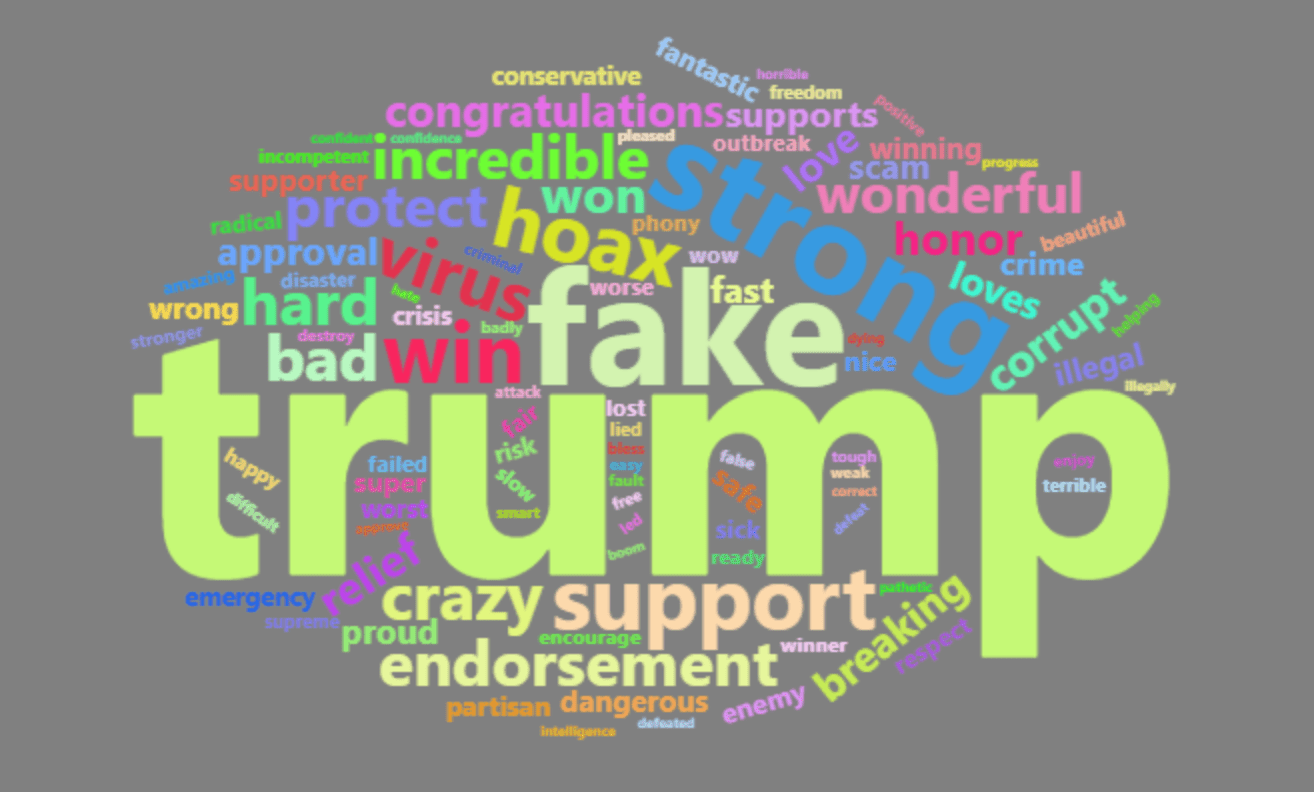
This week’s assignment was definitely one of my favorites – maybe even my favorite. I think the ability to analyze text and use word clouds to illustrate the results is absolutely incredible. I chose to analyze Trump’s Tweets; there were two options – Trump’s Tweets or Consumer Complaints. Regardless of political stance, I think that analyzing Trump’s Tweets is very interesting.

After importing the data (tweets from the past 3 months), we performed a number of tasks in order to determine Trump’s top twenty words in his tweets and then to separate these by sentiment – positive and negative. After this, we did a topic analysis. Some of these tasks were challenging, especially because this was a different sort of analysis. I did really enjoy it though! I will share an image for one of the word-clouds!

Week 12 – Proc and Roll with R

I was finally able to focus on R this weekend and catch up on all of my assignments. I spent a lot of time in R, and I definitely feel more confident in the program now. I was FaceTiming with one of my friends who has a lot of experience in R, and she was able to show me some things and help me fix my code in a couple spots. This week’s assignment was broken up into two parts – functions and clustering. We went back to our original red and white wine dataset and also utilized another wine dataset. I really enjoyed this assignment, and I walked away with a further developed R skillset.

The first part of the assignment utilized two datasets collected on red and white Portuguese wine. After importing the datasets, we had to join the datasets by wine color using bind rows. Then we created two different functions to use on our data. The first function mimicked PROC MEANS in SAS and provided the summary statistics. The second function mimicked PROC FREQ in SAS and provided the frequency and percent by variable. It took me a minute to get use to the format of the functions, but once I got it, it seemed pretty simple.

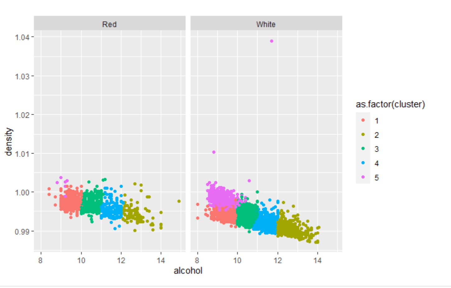
The final part of the assignment used our old wine dataset. After standardizing, we created some clusters for this wine data – using 5 clusters on alcohol, density, and residual sugar and separating red versus white wine.

I look forward to further developing my skills in R!

Week 11 – Regression Predictions

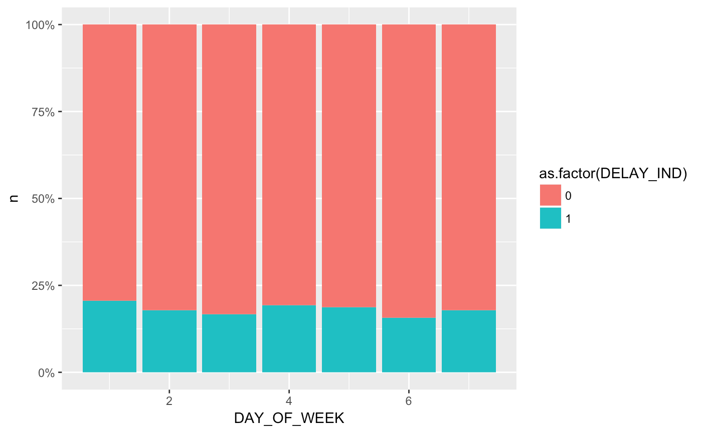
This week we continue our progression in R. This project is very interesting because it is about airline delays! The project looks at regression and estimation tasks with R’s Im function and modelr package. The goal is to perform estimation and regression modeling in a simplified way without using the “bread-and-butter” of regression. This project looks at flight delays overall and then looks at the possible contributing factors – day of the week effect, destination effect, and worst common flights.

This project is so interesting to me because I have often experienced delays and wondered about the contributing factors. Many can relate to flight delays, and the frustration they can cause! I am still getting use to R. It has taken me a bit longer to adapt to than SAS. I do like the platform, but the smallest thing can trip it up and it can take me a long time to determine how to fix it. I am looking forward to seeing where I am with it at the end of the class. It truly is such a useful tool!

Week 10 – Washington State Cannabis Sales and Regulatory Surveillance

I am still figuring out R. I know that the more and more time I spend in it, the more my confidence and knowledge will grow. Week 10’s assignment is very interesting. The data shows us Cannabis sales, inspections, and enforcement actions in Washington. This is so fascinating because this is such a hot topic and divided issue. Washington does not allow unlicensed cultivation for personal use, unlike other states that have legalized cannabis for recreational use. The industry is regulated by the state’s Liquor and Cannabis board and use has only been legalized for adults 21 and older. Given these restrictions, we are able to look at such great data.

This project delves into cleaning up the data, and then analyzing the sales top retailers, sales top counties 2016 versus 2017, sales top cities quarter one of 2017 versus quarter one of 2018, inspections by business 2016 and 2017, inspections by city 2016 and 2017, violations by business 2016 and 2017, and violations by type and city 2018. Lastly, the project takes a look at if inspections and violations are correlated and whether the day of the week matters for inspections or violations.

While I am still becoming comfortable with R and figuring out formatting issues, I think that this Project will move me in the right direction, and I am truly fascinated by the subject matter!

Week 9 – Midterm and R (Cont.)

I have been slightly behind due to being sick. I have basically finished my midterm. I feel confident in SAS, and I believe that my skills have really developed over the past several assignments. It is quite amazing to look back on my confusion and panic during the first week and to look at where I am at now. I look forward to using this Program in the future and honing in on my skillset further.

I have had a little bit of that same confusion and panic from the first week during this transition to R. It does appear to be very user friendly in a number of different ways. I do think that I may end up liking it more than SAS. I just need to take it all in and remember that I had the same initial feelings with SAS and look at how far I can in that. I really am looking forward to gaining more confidence in R and figuring out all the nuances. I really like how easy it is to access the libraries and import data. I also like how it holds on to what have you previously done. It also seems to very helpful in providing more guidance. More to come on this…

Week 8 – Midterm (Cont.)

The midterm has proven to be very challenging for me. I am still working on it. I think that the most difficult aspect of it has been translating the instructions into steps/tasks to complete. This assignment has definitely improved my thought process and independence in SAS though. It was a good assignment to end SAS. I have really enjoyed the challenge of putting together regression models for home values, especially given my passion for real estate.

I am looking forward to transitioning to R, but I know that it will bring new challenges. I am sure that it will be a bit of a transition to get use to the differences between the two programs.

Week 7 – Midterm – Predicting House Prices

The midterm combines bascially everything we have learned so far. It is definitely proving to be challenging because we have less help with this assignment. The prior assignments had a lot of example code, although we have had to rely on this less and less as we have progressed. I think that this assignment will definitely help with my independence and ability to rely on myself for these tough assignments.

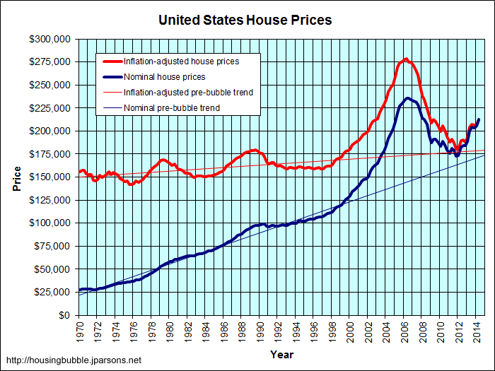
The midterm involves predicting home values for a major city in the United States. For this assignment, we will develop regression models to predict the home values. While this assignment does pose its own challenges, I find it very fascinating. I recently purchased a house, and real estate has sort of become a passion of mine. I have always found it interesting to look at what attributes make a house or property more valuable or a good investment. This assignment is right up my alley!

Week 6 – Regression & Estimation

We moved on from the Opioid data this week. We are looking at data from Wine. This week is very interesting to me because I love wine! We used this new data to carry out a few basic tasks. Then we added some new tools to our toolbox – we performed some T-Tests and some Regression Modeling.

I am definitely feeling more and more confident. The basic tasks are quite easy now, but sometimes the new tasks can be challenging until I have a good understanding. MACROS and some of the more complex work will need some more practice, but I think that is to be expected.

The simple tasks for this assignment compared white and red wines across several variables – including fixed acidity, citric acid, residual sugar, chloride, sulfur dioxide, density, pH, alcohol, and quality. There were about twelve in total. The descriptive statistics helped us compare white and red wines across these variables. We also compared and examined the correlations between these variables.

After these tasks, we moved on to the new tasks! The T-Tests seem to be pretty easy – we looked at alcohol content and quality for these. Then the regression models were definitely more complex. We did two different models – one predicted quality with citric acid, residual sugar, and alcohol; the other used more variables beyond these. We then compared these models to see which was better.

Picture: Example from this week’s PowerPoint